Recently, my Master’s program (UNH Analytics and Data Science, represent!) had a small module on webscraping using R via Rvest. I looked at a website called alltrails.com. It’s a really handy site for information on trails all around the world. I’ve only used it locally for New England trails, but I’ve seen trails in Spain pop up as well.
I’m an avid hiker. I’m originally from Maine, so I wanted to get a feel for the different trails in New Hampshire. New Hampshire has trails that range from a nice stroll to a strenuous hike up Mt. Washington. I had the thought that it would be cool to pick new trails based off the characteristics of previous trails that I had hiked–sounds like a good opportunity to cluster!
As is good web-scraping practice, I checked out the robots.txt file for the website. Some things were off limits for me, such as the website APIs and user info. But that’s alright, I only want information about the trails! Specifically, New Hampshire trails. I accessed the information needed from this specific webpage. On the right of the page is a loading bar for the best trails in New Hampshire, ranked from best to worst by the members of the alltrails community. Using RSelenium, it would be possible to load all the links via clicking the “Load” button repeatedly. Admittingly, I did not do this.
One day I’ll feel comfortable with RSelenium. For now though, I manually loaded the webpage side scroll and saved it to my local machine. From this local file, I scraped the links that would lead me to each individual trails site and the information that I needed.
So this link:

Gets me all this information:

You probably noticed a trail map of all the trails. I originally went to that map link to try and find latitude and longitude coordinates. Needless to say, I was unsuccessful in that endeavor. But I hit a lucky break: hidden away in the html source code of each link page are the latitude and longitude coordinates for the start of each trail. Here’s come example scode for how I pulled the links from the sidebar and pulled the relevant information from each link.
#Setting object to pipe through for trail urls
currentpage <- alltrails
#Piping through for the url of each trail that I want
trail_links <- currentpage %>%

 html_nodes("li.sortable") %>% #Going through each "sortable" node that's a trail

 html_nodes("a.item-link") %>% #going to that trail link

 html_attr("href") #pull the individual trail link
#Initializing empty lists to grab each trail Distance, Elevation, Route Type, Description, Name, and Difficulty
Distance <- c()

Elevation <- c()

Route_type <- c()

Description <- c()

Trail_name <- c()

Difficulty <- c()
#Looping through each link for the above attributes (but using html_text :)) in the first chunk
for(i in trail_link_1){

  trail_info <- read_html(i)

  distance <- trail_info %>%

   html_nodes("section#trail-stats") %>% #This section is pulling the distance from the web page

   html_node("span.distance-icon") %>%

   html_node("span.detail-data.xlate-none") %>%

   html_text()

Distance <- append(Distance, distance)

elevation <- trail_info %>%

  html_nodes("section#trail-stats") %>% #This one is pulling elevation

  html_node("span.elevation-icon") %>%

  html_node("span.detail-data.xlate-none") %>%

  html_text()

Elevation <- append(Elevation, elevation)

route_type <- trail_info %>%

  html_nodes("section#trail-stats") %>% #And this one is pulling route type

  html_nodes("span.detail-data") %>%

  nth(3) %>% # I couldn't get it to work without using "nth", something about detail data beginning the other trail stats

  html_text()

Route_type <- append(Route_type, route_type)

description <- trail_info %>%

   html_node("p#auto-overview.xlate-google.line-clamp-4") %>% #pulling the description

   html_text()

Description <- c(Description, description)

trail_name <- trail_info %>%

  html_node("div#title-and-difficulty") %>% #Grabbing the trail name

  html_node("h1.xlate-none") %>%

  html_text()

Trail_name <- append(Trail_name, trail_name)

trail_info <- read_html(i)

difficulty <- trail_info %>%

  html_nodes("div#difficulty-and-rating") %>% #Getting the difficulty

  html_node("span.diff") %>%

  nth(1) %>%  #Using nth again

  html_text()

Difficulty <- append(Difficulty, difficulty)

}
#Doing the same thing, but for latitude and longitude
Latitude <- c()
Longitude <- c()

for(i in trail_1){

 trail_info <- read_html(i)

 latitude <- trail_info %>%

  html_nodes("a#sidebar-map") %>%

  html_nodes("div") %>%

  html_node("meta") %>% #Navigating to this node had two "meta' lines: The first had the latitude

  nth(1) %>%

  html_attr("content")

Latitude <- append(Latitude, latitude)

longitude <- trail_info %>%

  html_nodes("a#sidebar-map") %>%

  html_nodes("div") %>%

  html_nodes("meta") %>% #And the second had longitude

  nth(2) %>%

  html_attr("content")

Longitude <- append(Longitude, longitude)

}
I elected to use the html source code rather than xpaths, as xpaths can change rather easily on a website. The nth() function is from Rtidyverse, and is really handy in this case. I constructed a dataframe from the info, and I was ready to cluster!
I elected to use python to cluster my trails dataframe. I ignored my Latitude and Longitide columns for clustering, as I didn’t want the trails to cluster on geographic information, only characteristics. I clustered on the continuous variables Distance and Elevation, and the categorical variables Route Type and Difficulty.
Route Type and Difficulty had three values each (Loop; Out & Back; and Point-to-Point, and Easy; Moderate; and Hard, respectively). By one-hot encoding this variables, I had 8 variables total. After standardizing them and running outlier analysis for 2% of the data, I identified by outliers.
Outliers

These trails are extradordinarily long–the type of trails that require a multi-day hike.
After outlier analysis, I ran PCA because why not? And I created 4 principle components that explained 90% of the variation in the data. Using K-Means Clustering (which most certainly is not the best clustering technique, but this isn’t an intense problem), I then ran a for loop to generate 5-12 clusters. I ended up selecting 6 clusters, as they seemed the most stable. From here, I loaded ggplot2 and leaflet to play around with map visaulizations.
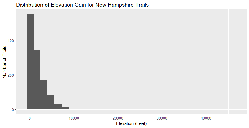
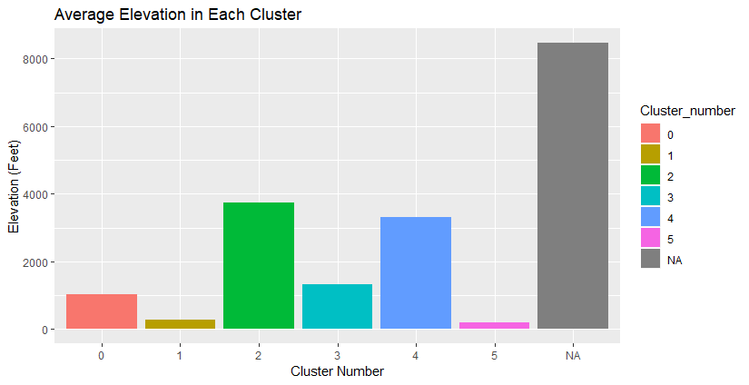
The elevation gain for most of these isn’t too intense, except for those really long trails. The tallest mountain in New Hampshire is a bit over 6000 feet, so this suggests that elevation gain measures the constant up-and-down of trails.
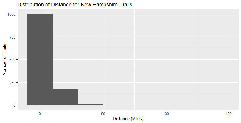
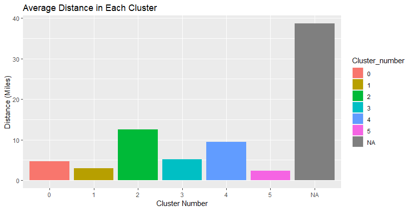
Most trails are under 25 miles, but there are a few exceptions (our outliers).

We see that the majority of the trails are of resonable length and distance, with a few outliers.
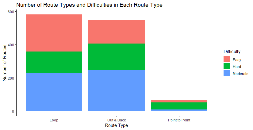
The most common types of routes are Loop routes and Out & Backs. Point-to-points aren’t as numerous.

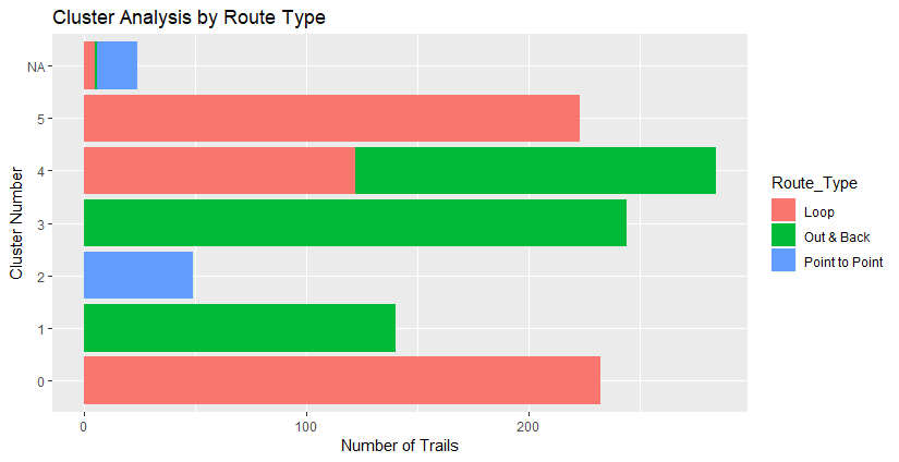
A side bar chart that illustrates the same info as the graph above.
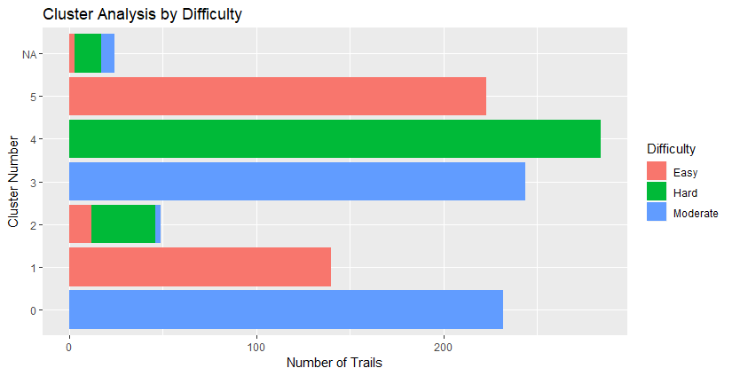
Below we start to get into the knitty gritty of it, and seeing the characteristics of our clusters.

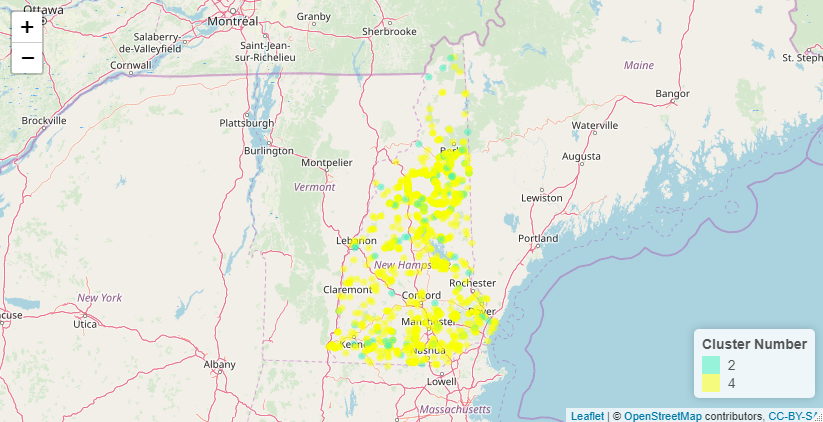
I plotted the clusters on leaflet to see where they’re located. Below is a map that has interactive pop-upsof trail descriptions, but I haven’t made them interactive on this website.

Below are all the clustered trails colored coded onto the map of New Hampshire. Here’s some example code for it:
#Creating colors for the clusters
clustercolor <- colorFactor(topo.colors(7), clusterdf$Cluster_number)
#Creating a leaflet for Clustered trails with their descriptions
z <- xx %>%
 leaflet() %>%
 addTiles() %>%
 addCircleMarkers(lat=xx$Latitude, lng=xx$Longitude, popup = ~Description,
               color = ~clustercolor(Cluster_number), fillOpacity = 0.6, radius = 0.3) %>%

Below is a similar map but only for the hard trails.
And these are the trails that are less than 3 miles.

Personally, I’m excited to “scrape” through the findings and use it a reference for the next trail that I want to hike! In theory, I can do this for multiple states, depending on my location.